Bands tutorial

In this section, we describe how to use Perturbopy to process a Perturbo 'bands' calculation.

The Perturbo 'bands' calculation interpolates the band structure using Wannier functions. The first step is to run Perturbo with calc_mode = 'bands'. More details can be found on the Perturbo website.

The YAML file used in this tutorial can be generated by following the Perturbo tutorial. The input files for this tutorial can be found here.

As described in the introduction we start by creating a Bands object si_bands to store all the information from the YAML file.

import perturbopy.postproc as ppy

si_bands = ppy.Bands.from_yaml('si_bands.yml')

The rest of this section is organized as follows. First, we explain how the data can be accessed from si_bands. Then, we explain how to perform calculations such as computing the direct bandgap, indirect bandgap, and effective mass. Finally, we explain how to plot the bands.

Accessing the bands data

Here, we describe how to access the data that is specific to the 'bands' calculation, which are the k-points and the interpolated band energies. Please see the Exporting data section for more information on accessing data general to all calculation modes, such as input parameters and material properties.

The outputs of the calculation are stored in two the Bands.kpt attribute and Bands.bands attribute, described in more detail below.

K-points

The k-points used for the bands calculation are stored in the Bands.kpt attribute, which is of type RecipPtDB. For example, to access the k-point coordinates and their units (which are column-oriented):

# Obtain the first k-point
si_bands.kpt.points[:, 0]

>> array([0.5, 0.5, 0.5])

# There are 196 k-points
si_bands.kpt.points.shape
>> (3, 196)

si_bands.kpt.units

>> 'crystal'

Please see the section Handling k-points and q-points for details on accessing the k-points through this attribute.

Band energies

The interpolated band energies computed by the bands calculation are stored in the Bands.bands attribute, which is a UnitsDict object. The keys represent the band index, and the values are arrays containing the band energies corresponding to each k-point.

# The keys are the band indices, and here we have 8
si_bands.bands.keys()
>> dict_keys([1, 2, 3, 4, 5, 6, 7, 8])

# Band energies of the 8th band
si_bands.bands[8]
>> array([13.69848506, 13.70154719, ..., 9.47676028, 9.46081004])

Please see the section Physical quantities for details on accessing the bands and their units.

Calculations

Direct bandgap

The direct bandgap is the difference between the valence band maximum (VBM) and the condunction band minimum (CBM), for which the k-vectors are the same. For example, to compute the direct bandgap in silicon between the valence band (band index 4) and conduction band (band index 5), we call Bands.direct_bandgap() with the two band indices as inputs:

# Compute the direct bandgap between bands 4 and 5
si_bands.direct_bandgap(4,5)

>> (2.513629987199999, array([0., 0., 0.]))

Bands.direct_bandgap() returns the bandgap, 2.51 eV, and the k-point at which that direct bandgap occurs, [0, 0, 0]. Note that silicon is an indirect bandgap material, so this is not the minimal energy difference between the valence band and conduction band.

Indirect bandgap

The indirect bandgap is the difference between VBM and CBM, without the same k-vector constraint. For example, to compute the indirect bandgap in silicon between the valence band and conduction band, we call Bands.indirect_bandgap() method with the two band indices as inputs:

# Compute the indirect bandgap between bands 4 and 5
si_bands.indirect_bandgap(4,5)

>> (0.4577520852000001, array([0., 0., 0.]), array([0.43137, 0.     , 0.43137]))

Bands.indirect_bandgap() returns the bandgap, 0.458 eV, the k-point of VBM is [0, 0, 0], and the k-point of CBM is [0.43137, 0., 0.43137].

Effective mass

The effective mass is computed in the parabolic approximation from the curvature of the parabola.

\[m^* = \frac{1}{{\frac{1}{{\hbar^2}} \frac{d^2E}{dk^2}}}\]

We can compute the effective mass of a carrier at band index n and k-point kpoint in the direction of the direction input. If no direction is provided, the longitudinal effective mass will be computed (i.e. the direction will be the same as the kpoint). Note that a direction must be provided if the k-point is [0, 0, 0].

Another important input is max_distance, which is the maximum distance from the central k-point to other k-points included in the calculation. For example, let’s compute the longitudinal effective mass at [0.43, 0., 0.43], which is the CBM of silicon. We will use max_distance of 0.12. The experimental value is ~0.98 :math:m_e

# Compute the effective mass of an electron at band 5, k-point [0.43, 0, 0.43]
# by a parabolic approximation that includes longitudinal k-points at a max
# distance of 0.12 from [0.43, 0, 0.43]
si_bands.effective_mass(5, [0.43, 0, 0.43], max_distance=0.12)

>> 0.9714141122114681

If an axis is provided, the band structure will be plotted, as well as the points chosen for the effective mass calculation and a dashed line reflecting the parabolic approximation (with a color specified by input c). Let’s plot the previous result.

import matplotlib.pyplot as plt

fig, ax = plt.subplots()

plt.rcParams.update(ppy.plot_tools.plotparams)

si_bands.effective_mass(5, [0.43, 0, 0.43], max_distance=0.12, ax=ax)

>> 0.9714141122114681

plt.show()

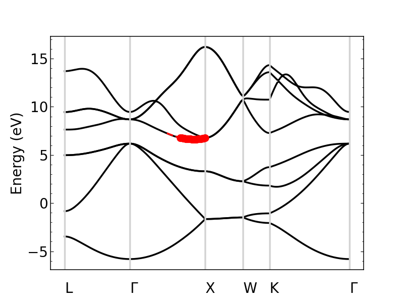
The plot shows the bands, with the points selected for the approximation plotted in red. Note that the points and line of fit stop at the “X” point because past here, the effective mass is no longer longitudinal.

We can zoom in to see the parabolic fit better. The dashed line is the parabolic fit, and extends past the points.

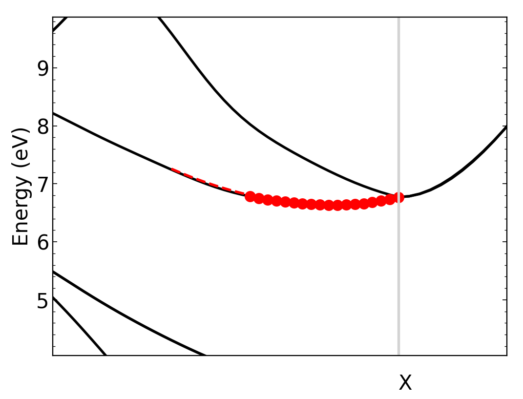
To increase the number of points used in the calculation, we should increase max_dist.

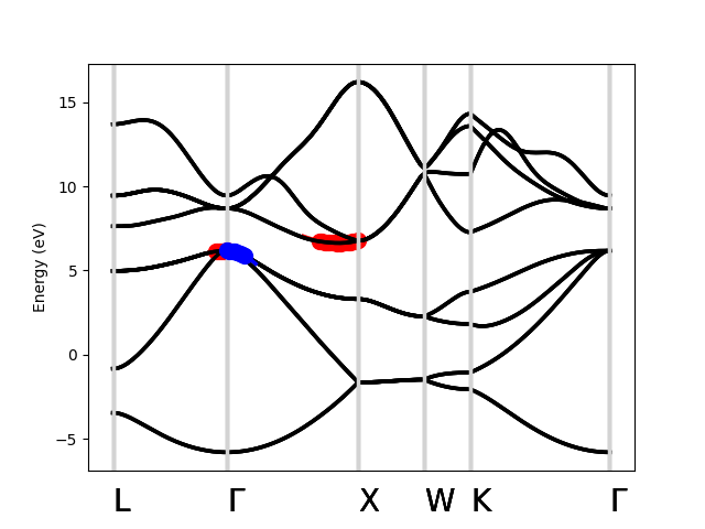
Next, let’s compute the effective mass for holes at the VBM (n=4, kpoint=[0, 0, 0]) in the [0.5, 0.5, 0.5] direction and [0.5, 0, 0.5] directions, which are the left and right effective masses, respectively. Note that, because this is a hole, we expect the effective mass to be negative.

m_left = si_bands.effective_mass(4, [0, 0, 0], max_distance=0.1, direction=[0.5, 0.5, 0.5], ax=ax, c="r")
m_right = si_bands.effective_mass(4, [0, 0, 0], max_distance=0.1, direction=[0.5, 0, 0.5], ax=ax, c="b")

m_left
m_right

plt.show()

>> -0.7826178453262155
>> -0.3391250154182139

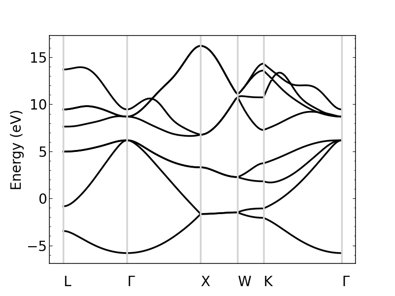
Plotting the band structure

Perturbopy allows users to quickly plot the band structure with a few lines of code:

import perturbopy.postproc as ppy
import matplotlib.pyplot as plt

fig, ax  = plt.subplots()

si_bands = ppy.Bands.from_yaml('si_bands.yml')

si_bands.plot_bands(ax)

For a nicer plot, we can use the plotparams dictionary provided in the plot_tools module. We can also add k-point labels (link to the k-point section) so that these are automatically added to the plot.

import perturbopy.postproc as ppy
import matplotlib.pyplot as plt

fig, ax  = plt.subplots()
plt.rcParams.update(ppy.plot_tools.plotparams)

si_bands = ppy.Bands.from_yaml('si_bands.yml')
si_bands.kpt.add_labels(ppy.lattice.points_fcc)

si_bands.plot_bands(ax)

Note that k-point labels can be removed from the plot by setting the show_labels input to False.

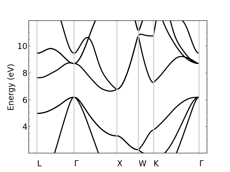
We can also change the energy window:

si_bands.plot_bands(ax, energy_window=[2,12])

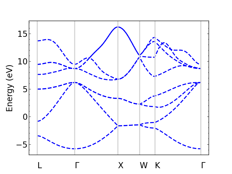
Other options include changing the linestyle and color.

si_bands.plot_bands(ax, c='b', ls='--')

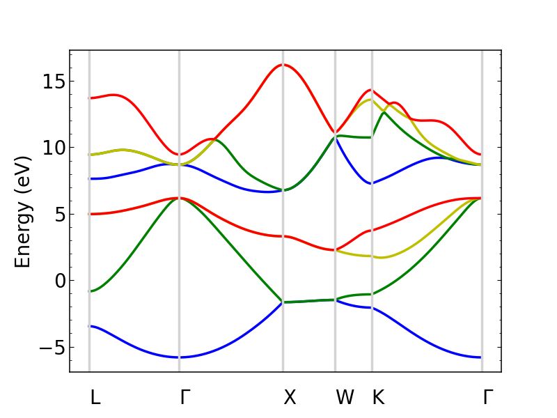
The colors and linestyles can also be a list.

si_bands.plot_bands(ax, c=['r','b','g','y'])