Dynamics-pp tutorial

In this section, we describe how to use Perturbopy to process a Perturbo dynamics-pp calculation.

The dynamics-pp calculation postprocesses the ultrafast dynamics calculations and computes the carrier population as a function of energy and time. Please see the Perturbo website for more details. We first run the Perturbo calculation following the instructions on the Perturbo website and obtain the YAML file, ‘si_dynamics-pp.yml’. We also obtain the popu HDF5 file ‘si_popu.h5’, which stores results from the dynamics-pp calculation too lage to be outputted to the YAML file.

Next, we create the DynaPP object using the YAML file and popu HDF5 file as an input. This DynaPP object contains all of the information from those two files.

import perturbopy.postproc as ppy

popu_path = "si_popu.h5"
yaml_path = "si_dynamics_pp.yml"

si_dyna_pp = ppy.DynaPP.from_hdf5_yaml(popu_path, yaml_path)

Accessing the data

The times are stored in the attribute DynaPP.times with units DynaPP.time_units.

si_dyna_pp.times

>> array([ 0.,  2.,  4.,  6.,  8., 10., 12., 14., 16., 18., 20., 22., 24.,
           26., 28., 30., 32., 34., 36., 38., 40., 42., 44., 46., 48., 50.])

si_dyna_pp.time_units
>> 'fs'

The energies are stored in the attribute DynaPP.energy_grid with units DynaPP.energy_units.

# There are 769 energies in the grid, corresponding to (emax - emin) / boltz_de
si_dyna_pp.energy_grid.shape
>> (769,)

# The first 4 energies in the grid
si_dyna_pp.energy_grid[:4]
>> array([6.63261242, 6.63361242, 6.63461242, 6.63561242])

# The units are eV
si_dyna_pp.energy_units
>> 'eV'

Finally, the populations are stored in the DynaPP.popu attribute.

# There are 769 energies in the grid and 26 time points
si_dyna_pp.popu.shape
>> (769, 26)

# The populations corresponding to the first 4 energies in the grid at the 25th time point
si_dyna_pp.popu[:4, 25]
>> array([0.00000000e+00, 0.00000000e+00, 9.45434167e-09, 4.15859811e-08])

Plotting the data

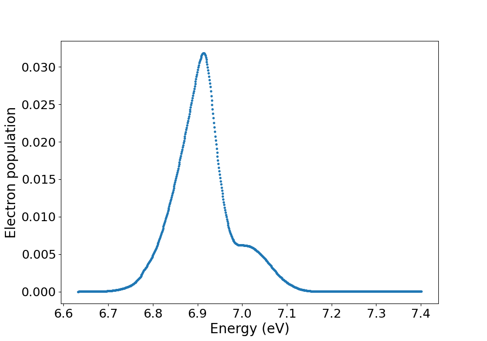
We can plot the carrier population function as a function of energy at a particular time point. Below, we plot it for the 25th time point.

import matplotlib.pyplot as plt

fig, ax = plt.subplots()

snap_number=25

plt.plot(si_dyna_pp.energy_grid,si_dyna_pp.popu[:, snap_number],marker='o',linestyle='', markersize=2.5)

plt.xlabel('Energy (eV)', fontsize = 20)
plt.ylabel('Electron population', fontsize = 20)
plt.xticks(fontsize= 18)
plt.yticks(fontsize= 18)

plt.show()