Phdisp tutorial

In this section, we describe how to use Perturbopy to process a Perturbo 'phdisp' calculation.

The 'phdisp' calculation mode interpolates the phonon dispersion by Fourier transforming real-space interatomic force constants. We first run the Perturbo calculation following the instructions on the Perturbo website and obtain the YAML file, ‘si_phdisp.yml’. For more information, please refer to the Perturbo website.

Next, we create the Phdisp object using the YAML file as an input. This object contains all of the information from the YAML file.

import perturbopy.postproc as ppy

si_phdisp = ppy.Phdisp.from_yaml('si_phdisp.yml')

Accessing the data

The main results of the results are stored in two objects:

• Phdisp.qpt stores the q-points used in the calculation

• Phdisp.phdisp stores the interpolated phonon energies computed

See Exporting data to learn how to access data from si_phdisp that is general for all calculation modes, such as input parameters and the material’s crystal structure.

Q-points

Phdisp.qpt is a RecipPtDB object that stores the q-points. For example, we can access the first q-points with the RecipPtDB.points property, which has the shape 3xN (where N is the number of q-points). Note that the q-points are column-oriented. For example, to access the first two q-points:

# Access the first two q-points
si_phdisp.qpt.points[:, :2]

>> array([[0.5   , 0.4902],
          [0.5   , 0.4902],
          [0.5   , 0.4902]])

# The points are a 3x206 array, as there are 206 q-points
si_phdisp.qpt.points.shape
>> (3, 206)

We can also access the units of the q-points:

si_phdisp.qpt.units
>> 'crystal'

Please see the section Handling k-points and q-points for more details on accessing information from Phdisp.qpt, such as labeling the q-points and converting to Cartesian coordinates.

Phonon energies

The interpolated phonon dispersion computed by the phdisp calculation are stored in the Phdisp.phdisp attribute, which is a UnitsDict object. The keys represent the phonon mode, and the values are arrays containing the phonon energies corresponding to each q-point.

# The keys correspond to phonon modes
si_phdisp.phdisp.keys()
>> dict_keys([1, 2, 3, 4, 5, 6])

# The values are arrays of phonon energies, of length N (the number of q-points)
si_phdisp.phdisp[6].shape
>> (206,)

# Phonon energies of the 6th mode
si_phdisp.phdisp[6]
>> array([60.26613499, 60.2667598 , 60.26863911, ..., 63.1558948])

Please see the section in the tutorial Physical quantities for more details on the UnitsDict object.

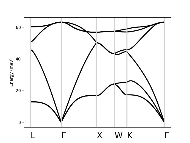
Plotting the phonon dispersion

We can quickly visualize the data by plotting the phonon dispersion.

import perturbopy.postproc as ppy
import matplotlib.pyplot as plt

# Create a figure and axis for plotting
fig, ax  = plt.subplots()

# Optional, used to format the plot
plt.rcParams.update(ppy.plot_tools.plotparams)

# Optional, used to label the q-points with labels for the FCC crystal structure.
# For example, [0.5, 0.5, 0.5] is the 'L' point in the FCC Brillouin zone.
si_phdisp.qpt.add_labels(ppy.lattice.points_fcc)

si_phdisp.plot_phdisp(ax)
plt.show()

For more information on how to customize this plot, please refer to the analogous section in the Bands tutorial, Plotting the band structure.