Ephmat tutorial
In this section, we describe how to use Perturbopy to process a Perturbo 'ephmat' calculation.
The ephmat calculation computes absolute values of the e-ph matrix elements, summed over the number of electronic bands, given two lists of k-points and q-points. We first run the Perturbo calculation following the instructions on the Perturbo website and obtain the YAML file, ‘si_ephmat.yml’. For more information, please refer to the Perturbo website.
Next, we create the Ephmat object using the YAML file as an input. This object contains all of the information from the YAML file.
import perturbopy.postproc as ppy

# Example using the ephmat calculation mode
si_ephmat = ppy.Ephmat.from_yaml('si_ephmat.yml')
Accessing the data
The k-points are stored in Ephmat.kpt, which is a RecipPtDB object. The data for the phonons is stored analogously in Ephmat.qpt (another RecipPtDB object) and Ephmat.phdisp, a UnitsDict object where the keys are the phonon mode and the values are the phonon energies computed across the q-points.
# Access the k-point coordinates. There is only one in this calculation.
# The units are in crystal coordinates.
si_ephmat.kpt.points
>> array([[0.],
          [0.],
          [0.]])

si_ephmat.kpt.units
>> 'crystal'

# There are 206 q-point coordinates (we display the first two below).
# The units are in crystal coordinates.
si_ephmat.qpt.points.shape
>> (3, 206)

si_ephmat.qpt.points[:, :2]
>> array([[0.5   , 0.4902],
          [0.5   , 0.4902],
          [0.5   , 0.4902]])

si_ephmat.qpt.units
>> 'crystal'

# Access the phonon energies, which are a UnitsDict.
# There are 6 modes, which are the keys of the dictionary.
si_ephmat.phdisp.keys()
>> dict_keys([1, 2, 3, 4, 5, 6])

# Phonon energies of the first 2 q-points in phonon mode 3
si_ephmat.phdisp[3][:2]
>> array([45.69220981, 45.61860655])

si_ephmat.phdisp.units
>> 'meV'
Please see the section Handling k-points and q-points for more details on accessing information from Ephmat.kpt and Ephmat.qpt, such as labeling the k, q-points and converting to Cartesian coordinates.
The ephmat calculation interpolates the deformation potentials and e-ph elements which are stored in dictionaries Ephmat.defpot and Ephmat.ephmat, respectively. Both are UnitsDict objects. The keys represent the phonon mode, and the values are (num_kpoints x num_qpoints) size arrays.
# There are 6 keys, one for each mode.
si_ephmat.ephmat.keys()
>> dict_keys([1, 2, 3, 4, 5, 6])

# There is 1 k-point and 206 q-points, so the e-ph matrix is 1 x 206.
si_ephmat.ephmat[1].shape
>> (1, 206)

# The e-ph matrix elements corresponding to the first phonon mode,
# first (and only) k-point, and first two q-points.
si_ephmat.ephmat[1][0, :2]
>> array([[11.80265941, 11.92405409]])

# The units are in meV.
si_ephmat.ephmat.units
>> 'meV'

# We can extract analogous information from the deformation potential.
si_ephmat.defpot[1].shape
>> (1, 206)

si_ephmat.defpot.units
>> 'eV/A'
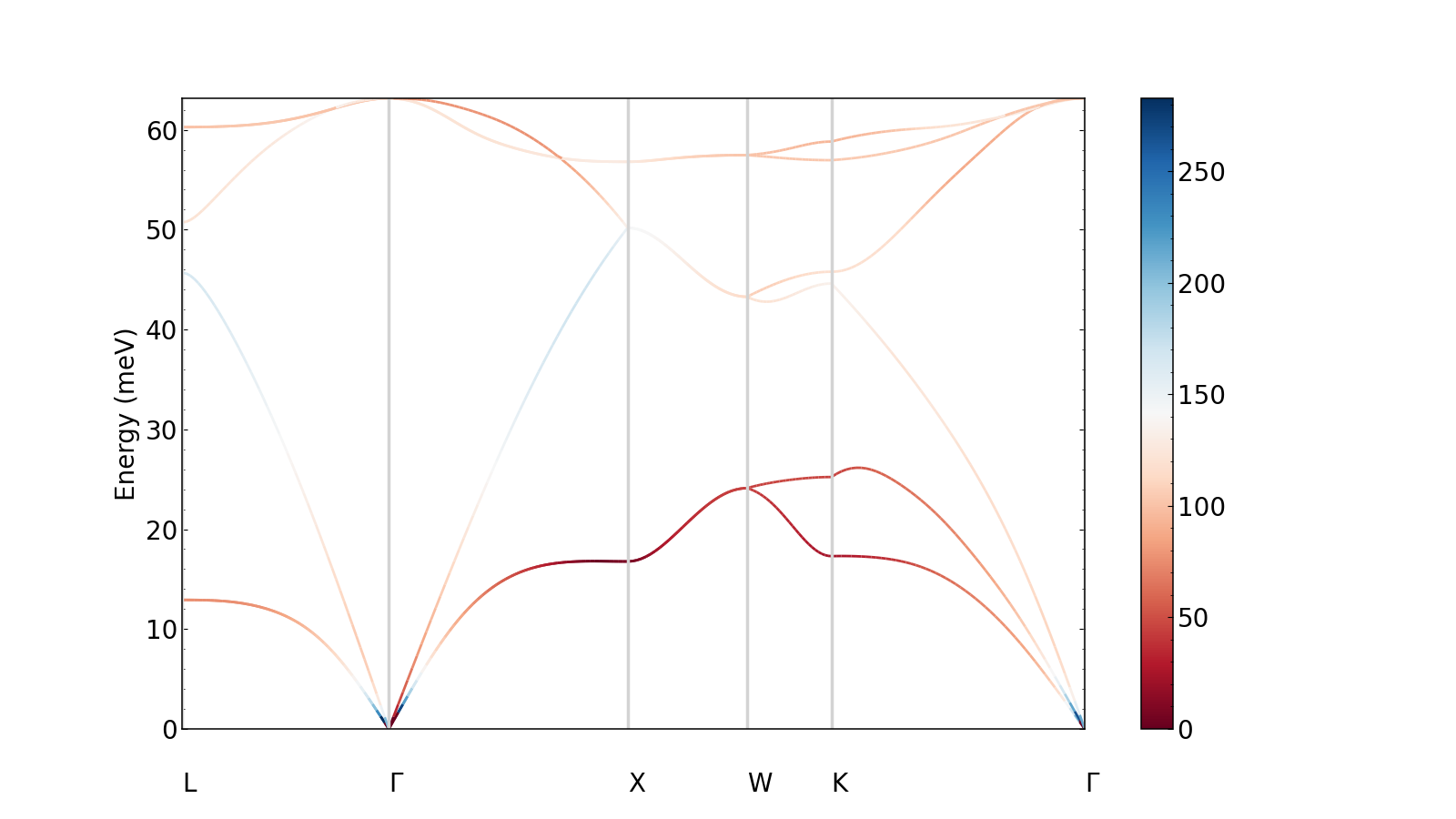
Plotting the data
We can quickly visualize the e-ph elements by plotting them as a colormap overlaid on the phonon dispersion. Below, we plot the e-ph elements computed at the k-point [0, 0, 0] along the q-point path.
import matplotlib.pyplot as plt

plt.rcParams.update(ppy.plot_tools.plotparams)
si_ephmat.qpt.add_labels(ppy.lattice.points_fcc)

fig, ax  = plt.subplots()
si_ephmat.plot_ephmat(ax)
plt.show()
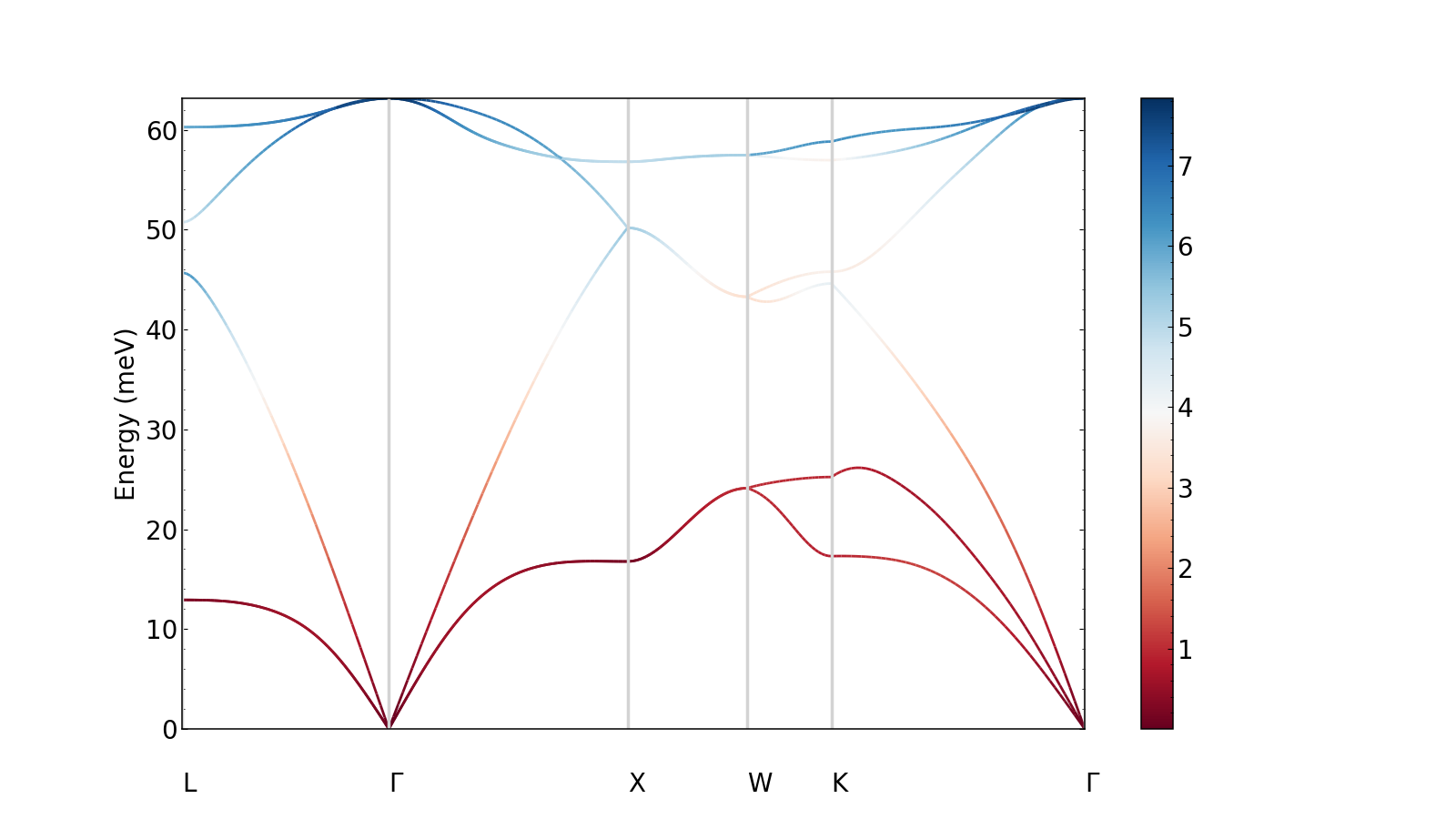
We can also plot the deformation potential instead.
si_ephmat.plot_defpot(ax)
plt.show()
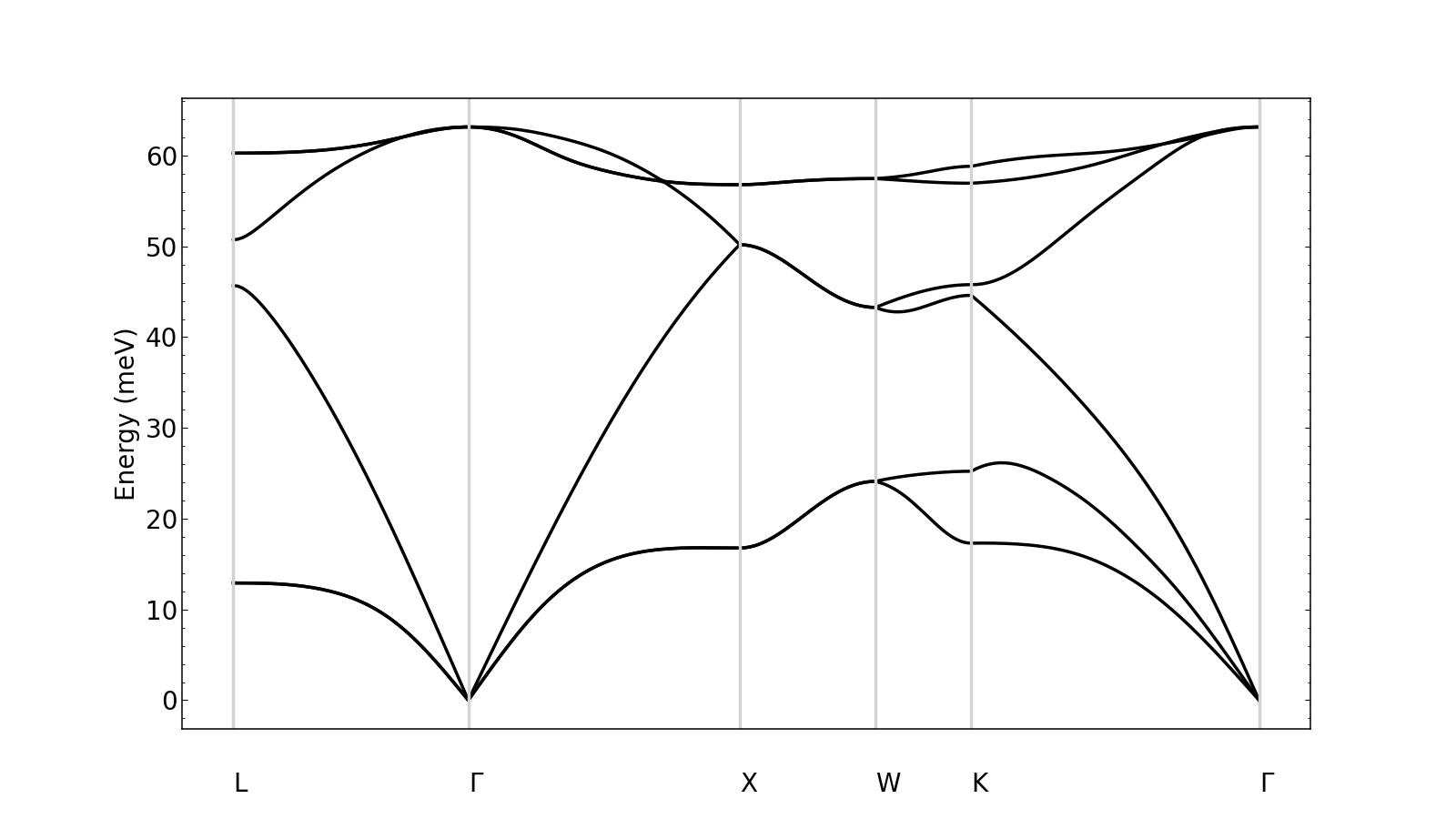
Finally, if we want to plot simply the phonon dispersion,
si_ephmat.plot_phdisp(ax)
plt.show()
If we performed the 'ephmat' calculation with multiple k-point as well as q-points, we can choose the k-point for which we plot the e-ph elements or deformation potentials across all the q-points.
For example, let’s say we repeated the calculation, but with three different k-points. The q-points remain the same.
si_ephmat_expanded = ppy.EphmatCalcMode.from_yaml('si_ephmat_expanded.yml')

si_ephmat_expanded.kpt.points

>> [[0.  0.  0. ]
    [0.5 0.5 0.5]
    [0.5 0.  0.5]]
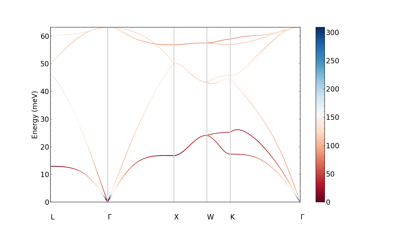
Now when we plot the e-ph elements, we can choose whether we want to plot them for the first, second, or third k-point by setting kpoint_idx. For example, let’s plot results for the third k-point, [0.5, 0.0, 0.5]. (By default, the first k-point is used.)
plt.rcParams.update(ppy.plot_tools.plotparams)
si_ephmat_expanded.qpt.add_labels(ppy.lattice.points_fcc)

fig, ax  = plt.subplots()
si_ephmat_expanded.plot_ephmat(ax, kpoint_idx=2)
plt.show()